
Understanding Field Weakening Pt. 1

Foreword
This article is for Charlie Seifert. He casually requested a write-up about field-weakening in the comment section of the reactive power piece I wrote earlier.
Initially I was on the verge of quoting his comment and simply say that:
“Field-weakening is just what happens when a converter runs out of voltage and is unable to sustain a nominal field across the air gap, and this will limit the capacity for torque production”.
After some consideration, this answer left me thinking: What is the field, really? And why does it impact the torque? When does this happen? What do we do about it? What about different types of electrical motors, how do they respond? What can the inverter do?
These questions kept me awake, and I realized I did not understand this issue well enough. Heck, I didn’t even understand the fundamentals of magnetism inside the machine. And so, this article is both to understand it myself and hopefully make you understand it as well.
So, thanks Charlie. I needed this.
We needed it.
Introduction
The term field weakening is known by all who design electrical motors and variable speed drives (VSD) and by many who have commissioned them. But its actual meaning, cause and consequences are often somewhat blurry. At least if you’re not a motor designer.
In short, it can be described as the result of voltage starvation; the faster the motor runs, the more voltage it requires to maintain its nominal magnetic field strength. So when increasing the motor speed, it will eventually require more voltage than the VSD is able to deliver.
In some ways we can also describe it as a voltage fight between the motor and its VSD:
Every converter has a maximum output voltage
↓
A motor will fight back the output voltage with its back-EMF
↓
The back-EMF increase with speed
↓
Eventually, voltage from back-EMF reaches the VSDs maximum voltage
↓
To further increase speed a compromise is needed:
↓
Either, the motor will fail to carry its load, or the speed must be reduced
Field weakening is normally not an issue when using VSDs with sufficient AC supply voltage when running at (or below) the motor’s nominal speed. Nor is it an issue for directly grid-connected motors being supplied with their nominal voltage and frequency.
However, connecting a motor designed for 440V 50 Hz to a 400V 50 Hz outlet will put the motor firmly in a constant state of field weakening.
This article will cover field weakening caused by VSD operation above rated motor speed. I will try to explain why it occurs and the effects of it.
But it is impossible to truly understand field weakening without truly understanding The Field.
Hence, this article will start by understanding the magnetic fundamentals of electrical motors as well. Sorry. Blame Charlie.
Below is an outline of how this article will proceed:
Part 1: The Induction Machine and its Magnetic Field – from scratch
The parts a motor consists of
The magnetic circuit, windings and rotating fields
How magnetism in iron work, and the damn saturation
Magnetomotive forces, The magnetic field and back-EMF
How the magnetic field creates torque
Part 2: More Torque!
What affects torque / torque characteristics
FEM-analyses
TBA
Also TBA
Part 3: Field Weakening Scenarios using VSD
Part 3a: Scalar controlled induction motor; VSD output is a V/f curve to the motor
Part 3b: Vector controlled induction motor; both torque and flux is tightly controlled by VSD
Part 3c: Vector controlled permanent-magnet motor: flux from factory, torque from VSD (I suspect this is the thing Charlie was after, but I am not sure)
The two main questions in these three scenarios are: “Where does the flux come from?”, and “Who controls it?”
The complexity of these questions increases through these three scenarios, but let’s start in the shallow end, shall we?
Table of Symbols / Nomenclature
I know this sounds scary, but at least you know where to look when strange symbols start to appear in the text and equations
Magnetic stuff
ϕ - Magnetic flux
λ - Winding flux linkage
H - Magnetic field strength (as created by ampere-turns)
B - Magnetic flux density (the result after taking the material into account)
M - Magnetization of the material
μ0 - The magnetic permeability of vacuum; in Henry pr meter.
μr - The relative permeability of a material. Air = 1, Stator Iron; typically 2000-5000.
μ - Combined permeability; μ=μrμ0
F - Magnetomotive Force, MMF - Creates H .
R - Reluctance (magnetic resistance), opposes flux
ℓ - The length of a magnetic material, used to calculate H=F/ℓ
Motor symbols
f - Frequency. Supplied to the motor.
s - Slip Speed. Difference between the stator synchronous speed and rotor rotational speed.
p - Number of pole pairs
n - Number of winding turns
kw - Winding factor in the stator. A factor between 0 and 1 to take into account that as windings are distributed in discrete slots, they are not perfectly positioned to establish a sinusoidal waveform, and some fundamental EMF/MMF is lost.
π - This you know.
Electrical components in the motor equivalent models
e - Back-EMF. The voltage-drop created by the inductance in the windings.
V1 - is the applied winding voltage per phase
Is - represents the main stator current
R1 - is the stator winding resistance
jX1 - is representing the stator leakage flux (which is not linked to the rotor)
I0 - is no-load current or magnetizing current
Rc - are the magnetic core losses (eddy currents, hysteresis)
jXm - is the air gap magnetizing reactance (this is an important one)
jX′2 - is the rotor reactance
I′2 - is the rotor current
R′2(1−s)s - is the slippage dependent rotor resistance
The Induction Machine and its Magnetic Field
This article will cover both induction machines and permanent magnet (PM) motors, but the first one is the beautiful one and when we understand that one, the PM motor comes more easily. So, for now, let us dig into the induction machine. And we will do this from scratch. To understand the field - you must become the field.
Construction of a squirrel cage induction machine
The induction machine is designed to create and carry magnetic fields. The field creates a twisting force (torque) to rotate the shaft.
It is constructed with amazingly few parts, is simple to assemble and can easily outlive a human. I would argue that the induction motor is the electric equivalent to a Kalashnikov; you can throw it in a swamp and pick it up twenty years later, and it will still work after brushing it of.
In this article, I will first present “all” the parts, and when they are shown, described and accounted for, I will throw away all the passive parts and continue with the parts that matter. “Passive” mean that they are not related to the magnetic field and torque production.
Passive Parts
Housing (to live inside)
End-cover (ingress protection)
Bearings (to hold it in place, but allow rotation)
Fan (to(o) cool)
Fan-cover (to protect fingers etc)
Connection house (to connect supply cable)
Mount (to fasten the thing so it doesn’t tip over)
Screws (to hold it together)
Shaft (to make use of the rotation)
Slot liner (protection and isolation of windings in the stator slots)
Active Parts
Stator laminations (steel for magnetism)
Stator windings (copper for current)
Rotor bars (copper or aluminum, also for current)
Rotor laminations (steel, also for magnetism)
Rotor end-rings (to short circuit rotor bars)
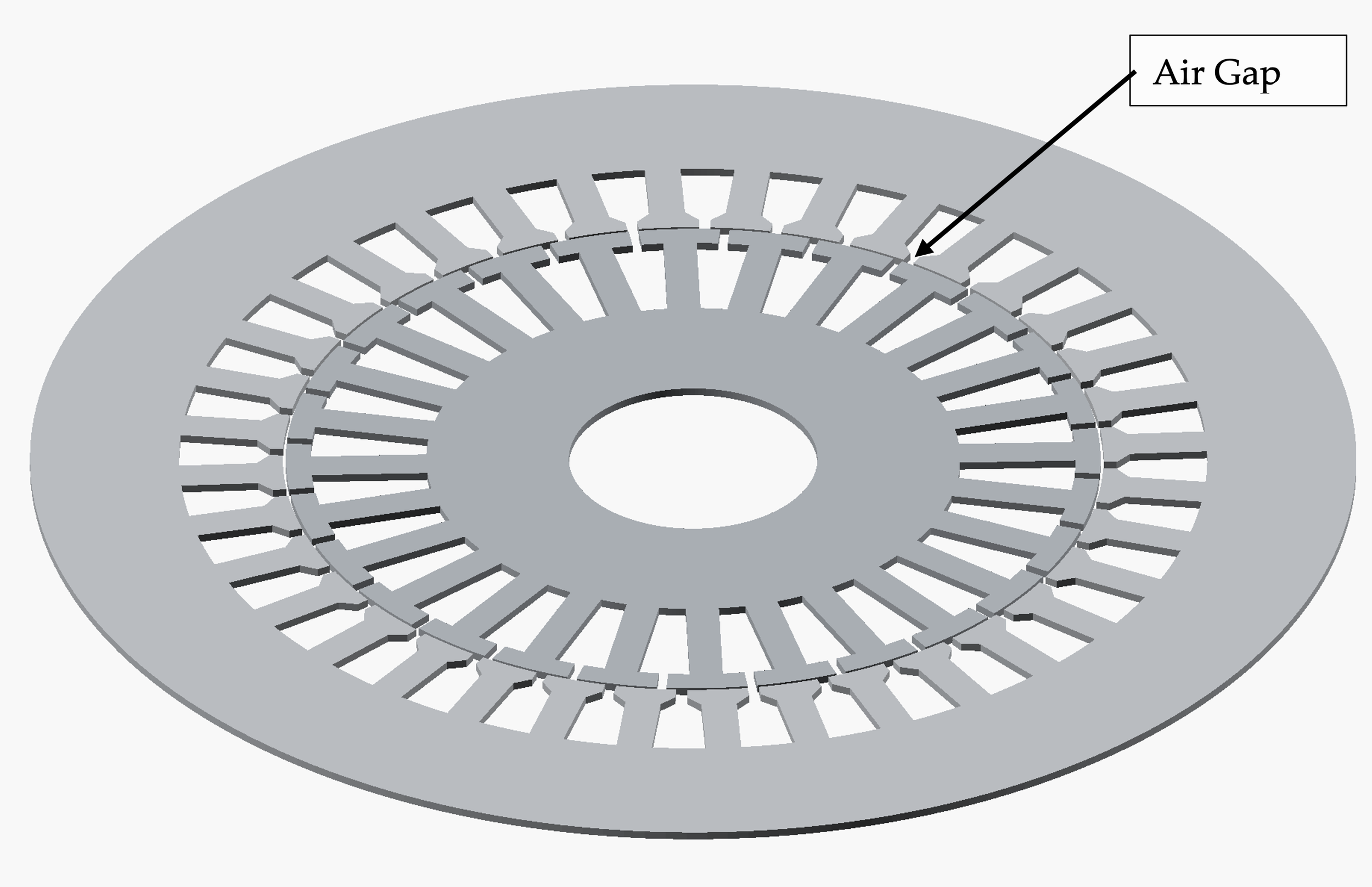
Air gap (well, not actually a “part” - but a damn important feature)
That’s all. I think…
Below I have presented some photos of a piston pump motor I actually went ahead and found in cold storage at work and disassembled for your viewing pleasure. I had to carry it half a mile back to my workstation. Hope you’re happy, Charlie.
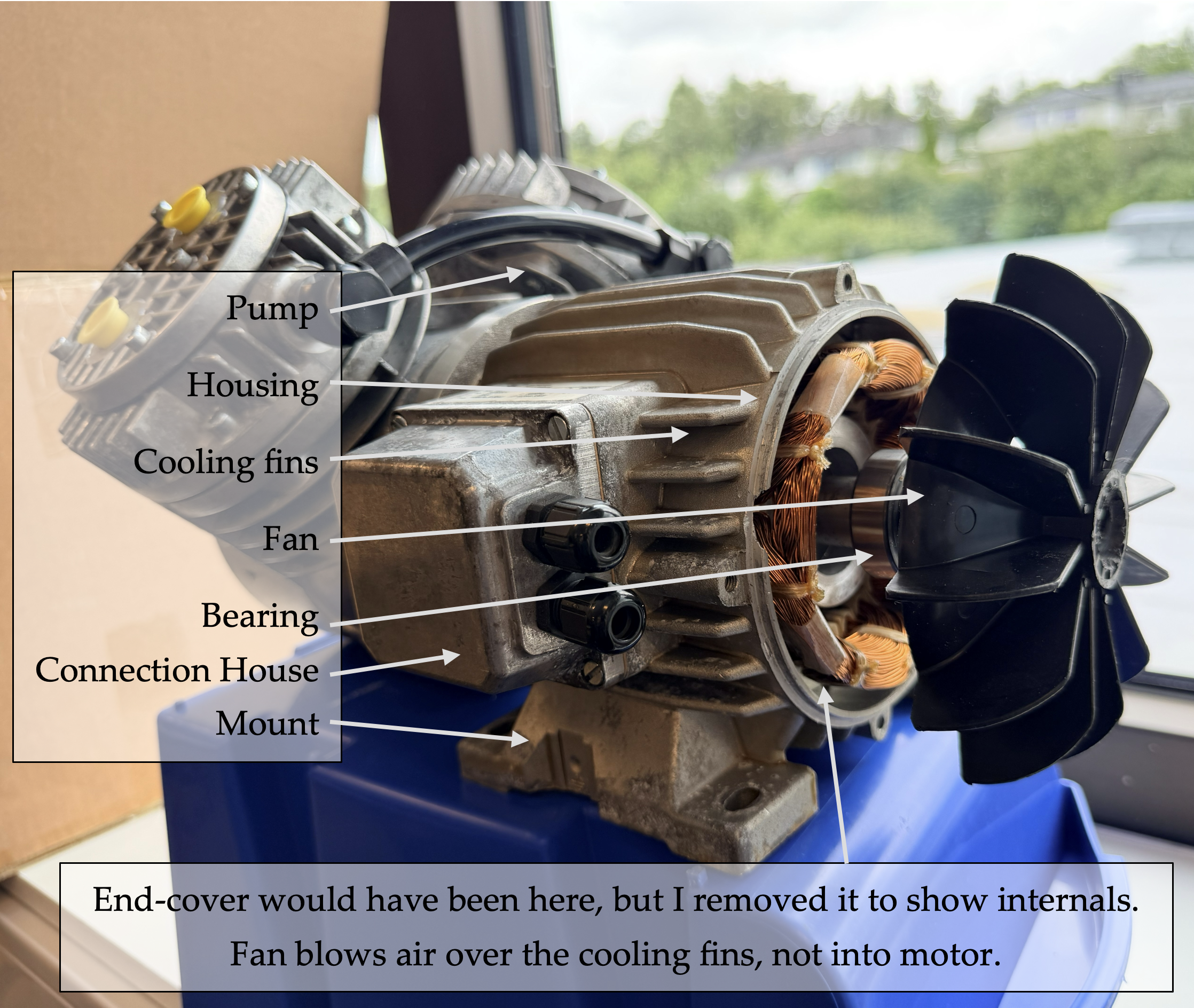
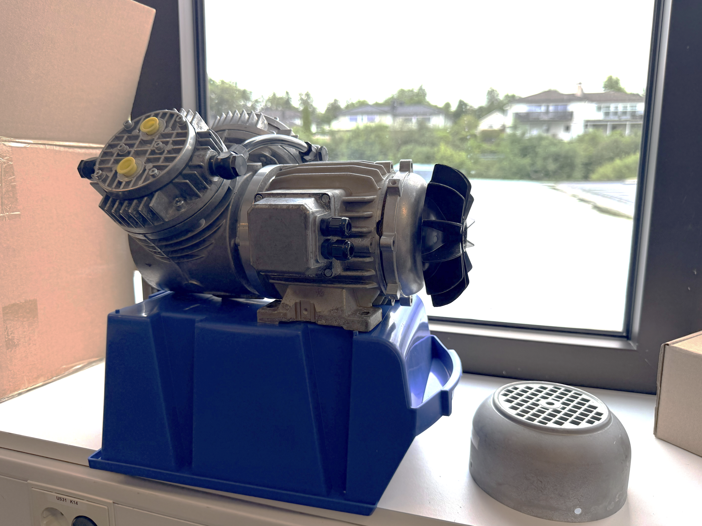
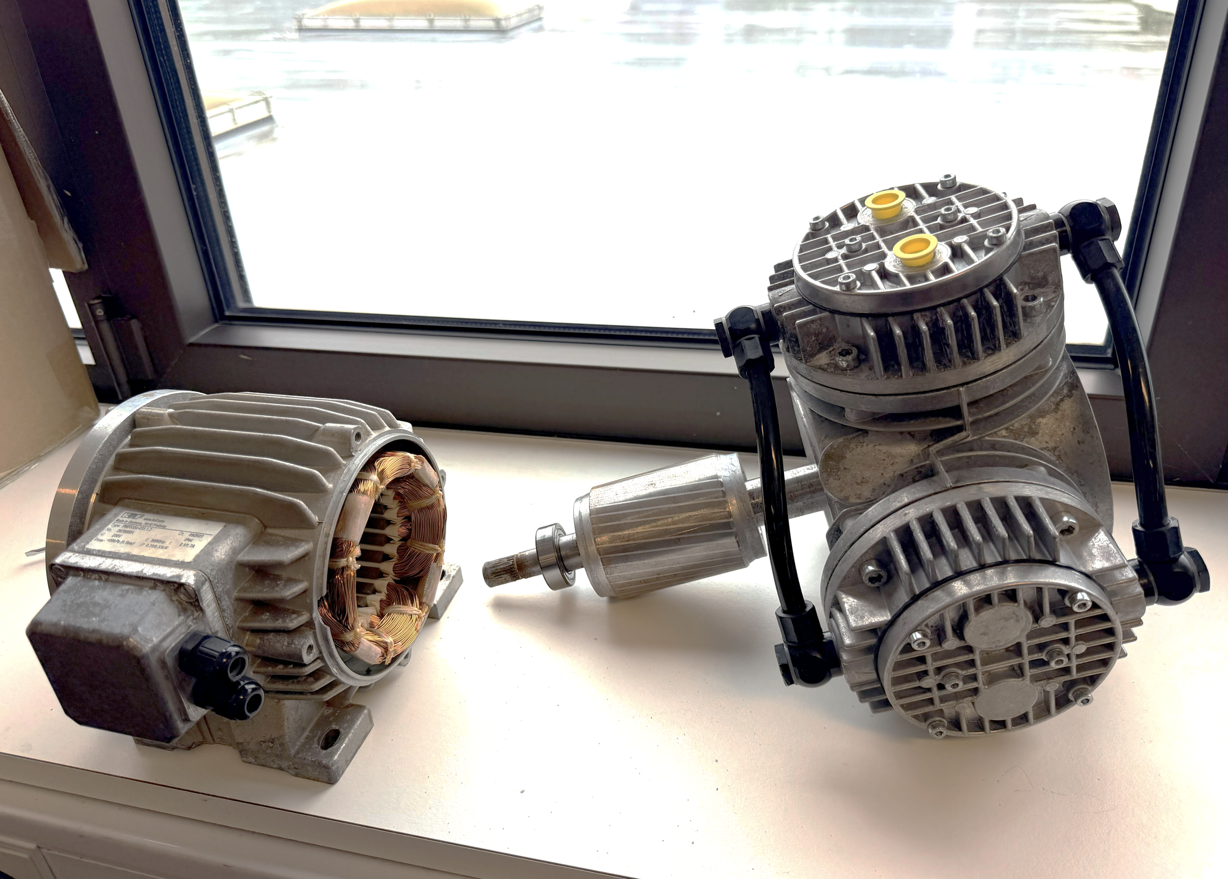
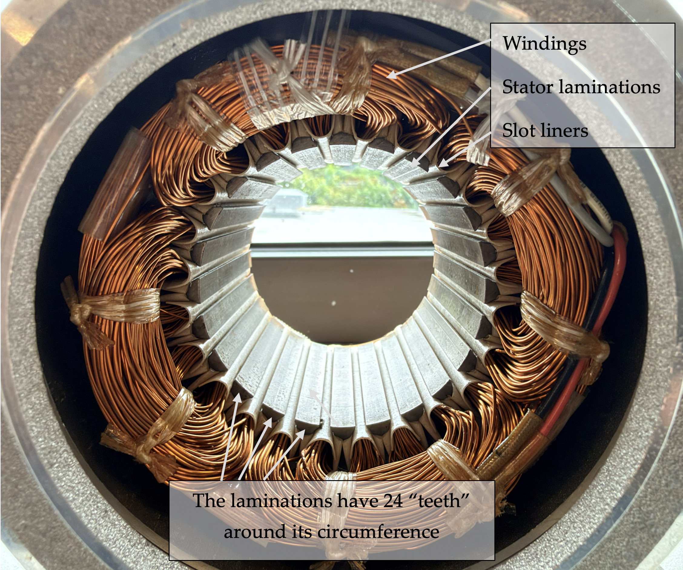
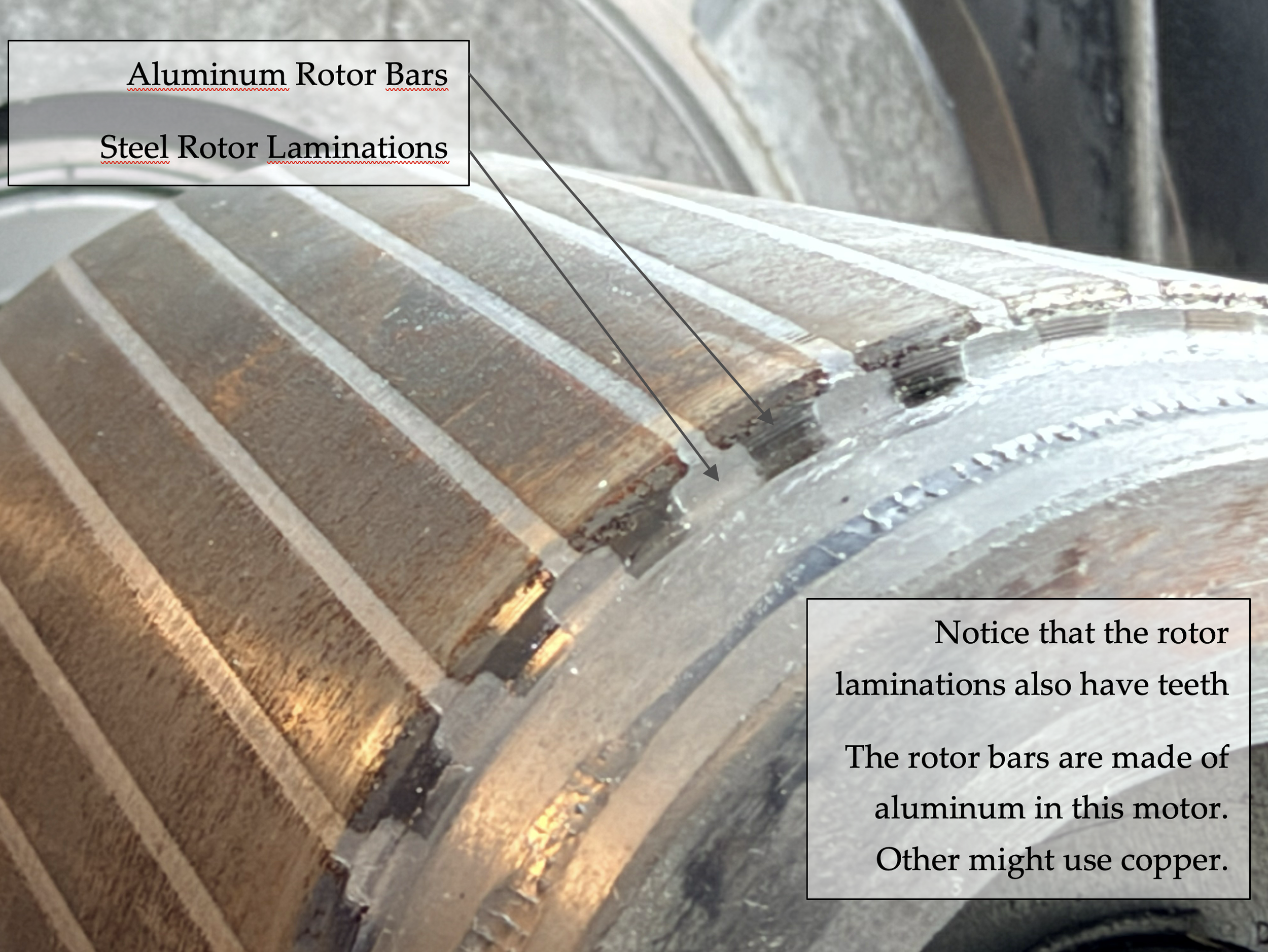
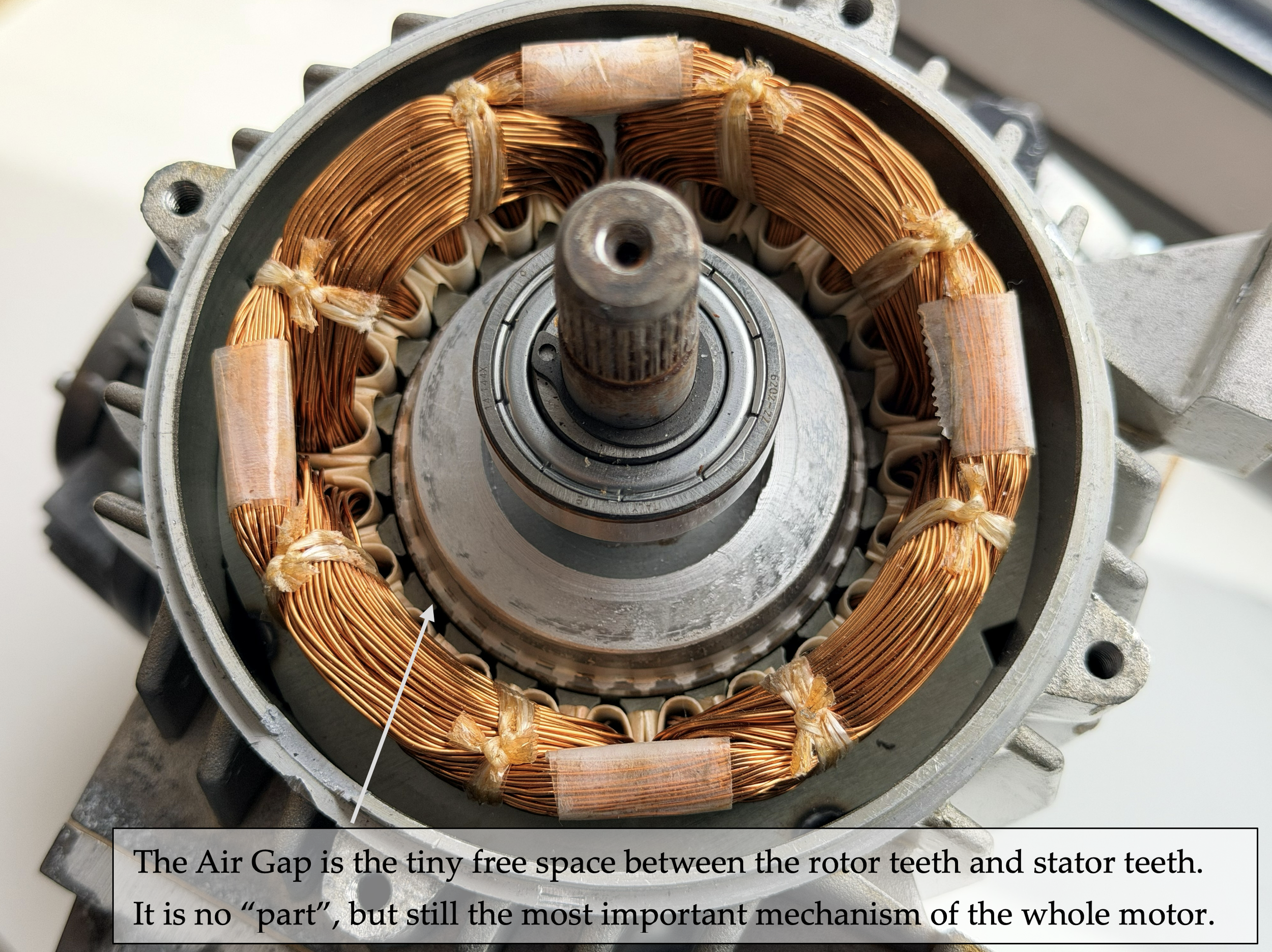
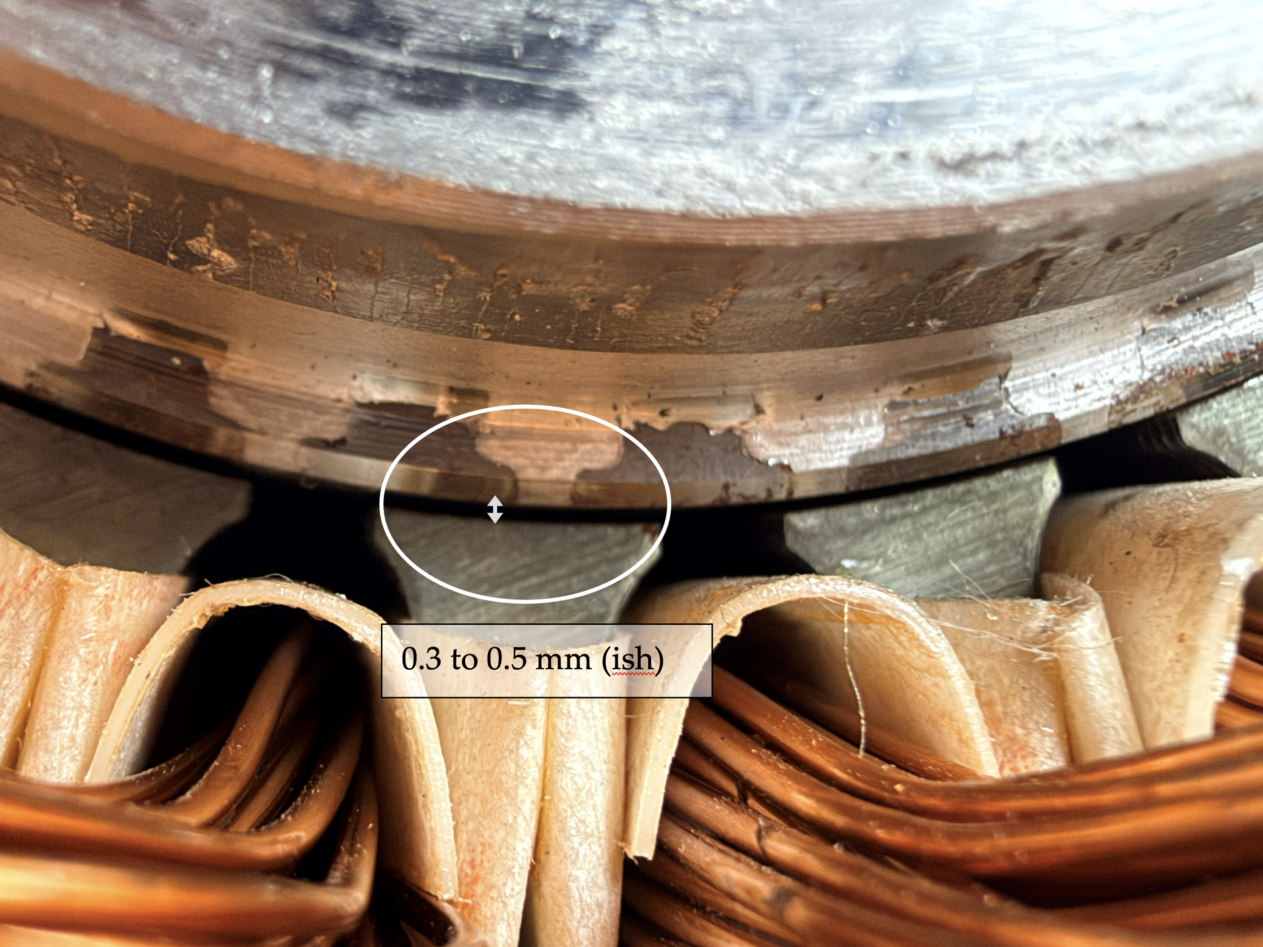
To further illustrate the induction motor, I found the original CAD drawings of the pump, and designed a similar stator and rotor using OpenSCAD (the pump CAD drawings didn’t bother to include such details, after all it’s a pump, not a curriculum)
The rotor lives inside the stator, which lives inside the stator bore of the housing. Just like matryoshka dolls.
I forgot to include the actual shaft though, it is suppose to come out of the rotor so that the rotation can be used by something connected to it.
When we pull out the rotor and the stator from the housing, we are left with the passive parts we are now saying good bye to as we are leaving all these “nice to have” parts behind to focus on the electrical and magnetic stuff.
The stator and rotor’s purpose is to create or accommodate two different “pathways”:
Iron laminations to carry the magnetic flux,
and…current carrying windings to create it.
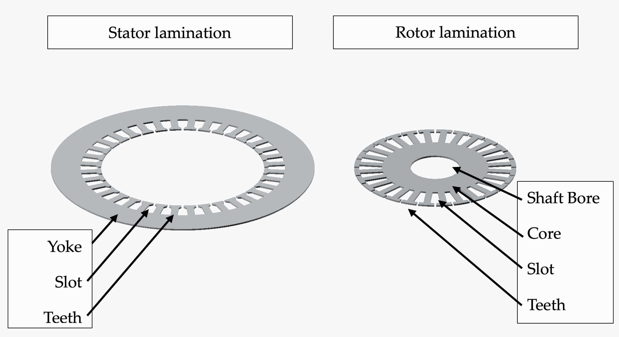
Below we will examine the iron laminations which form the stator and rotor stacks. They are here shown next to each other. Both laminations consist of three sections with their own name worth explaining.
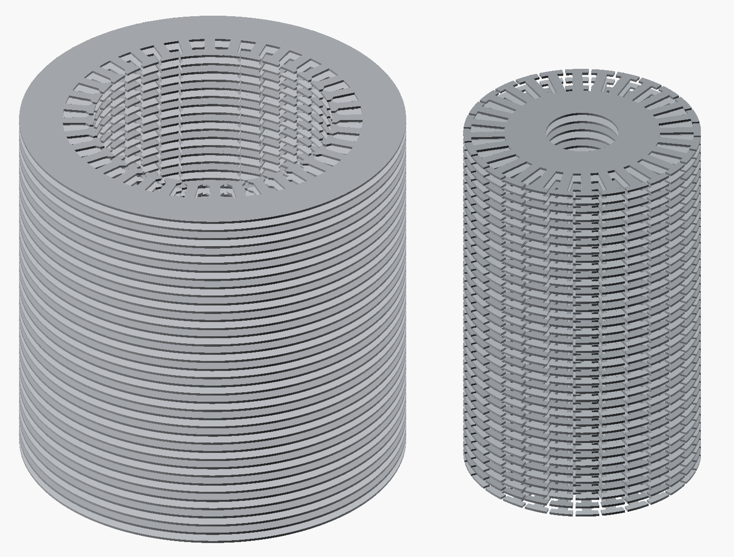
The whole rotor and stator consist of many such laminations; usually hundreds. They are all coated with an insulating layer on both sides to limit the extent of eddy currents in the iron as this is pure loss. When the machine is built, these laminations are pressed tightly together.
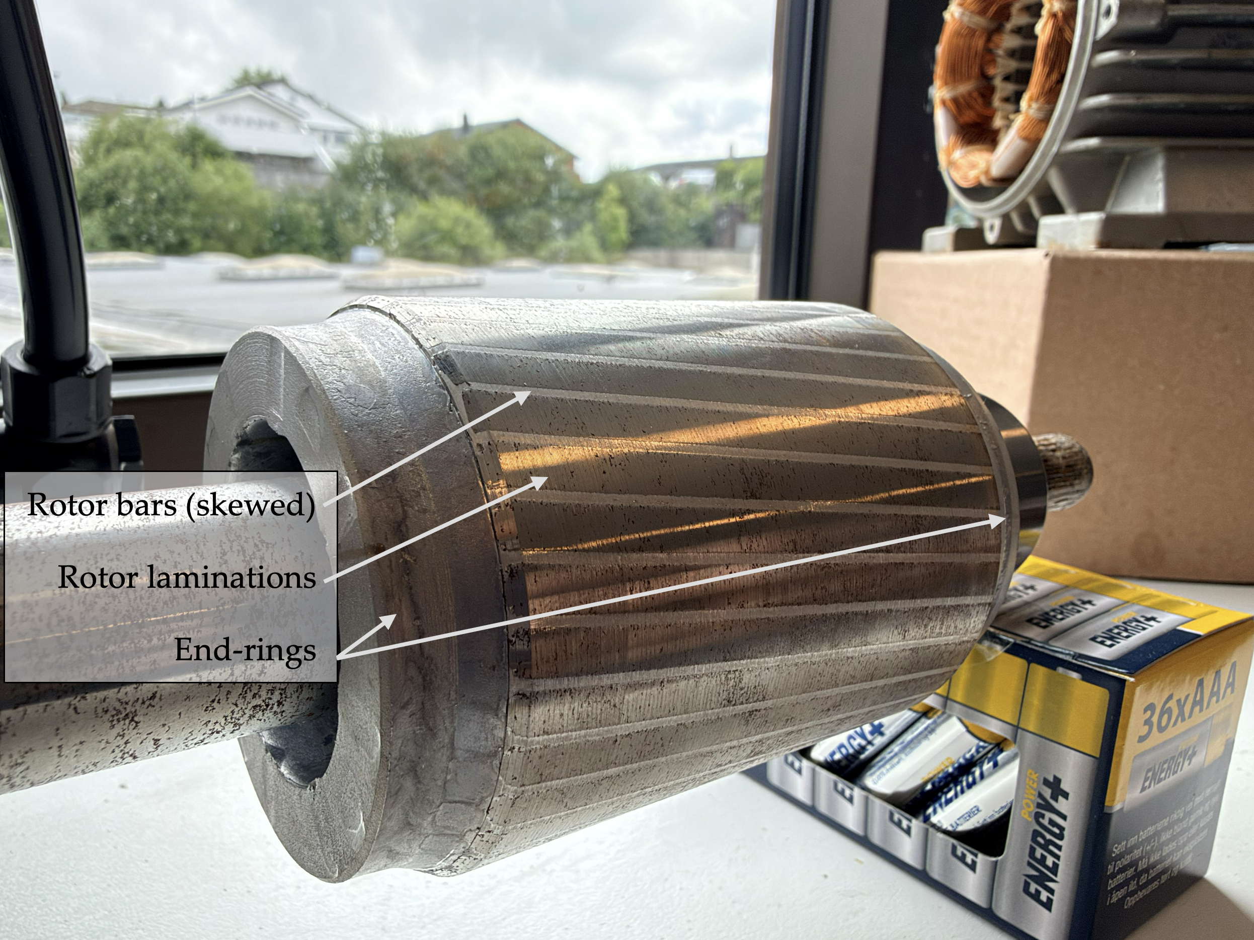
Below are images of the rotor bars. These are usually made of aluminum or copper. In the photographs above, only the narrow outer tip was visible, but here you can see how they extend deeper into the rotor. Later, we will learn how the depth and form of the rotor bars are designed to manipulate the relationship between resistance and inductance, and further how that relationship defines the motor’s torque characteristics.
The rotor is shown in four different settings:
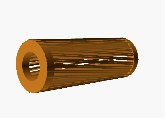
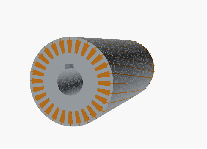
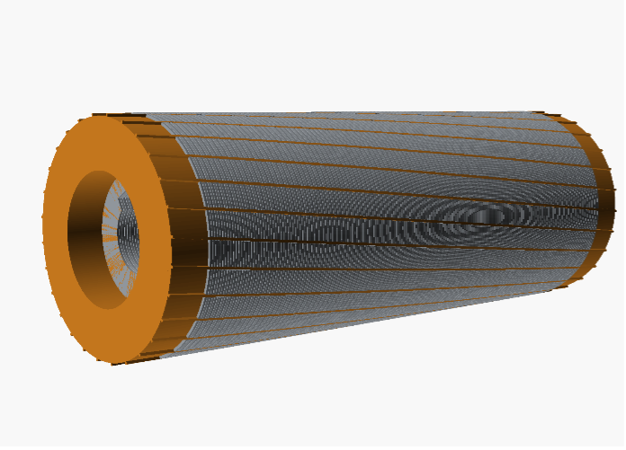
The end-rings’ purpose is to short-circuit the end of all rotor bars. When I was a student, I could not comprehend how there could flow any current in them due to this. Later, we’ll learn how. You will also notice that the bars are skewed. We will explain this too. For now, just remember that it has a purpose.
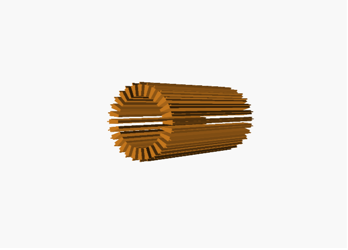
Below, I am showing how the two parts are assembled into a complete stator stack and rotor stack.
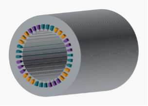
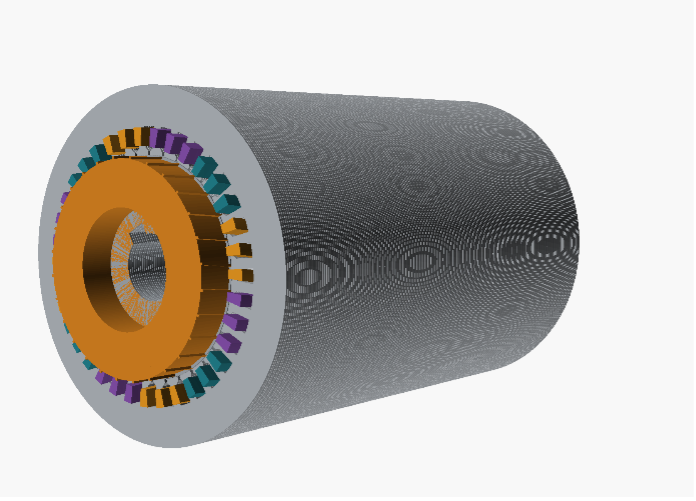
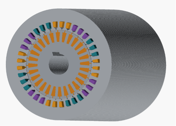
The green, purple and orange “sticks” pointing out are the windings. These are in three different colors because there are three phases.
In a real motor (and in the photos earlier), they usually look like a mess of wires bundled together and fastened with string. At this point we are not showing how they are connected to each other, but I can reveal that this is a four-pole machine because each color appears four times.
Moving from photos to CAD to finally reaching the most common format in the literature: TikZ figures:
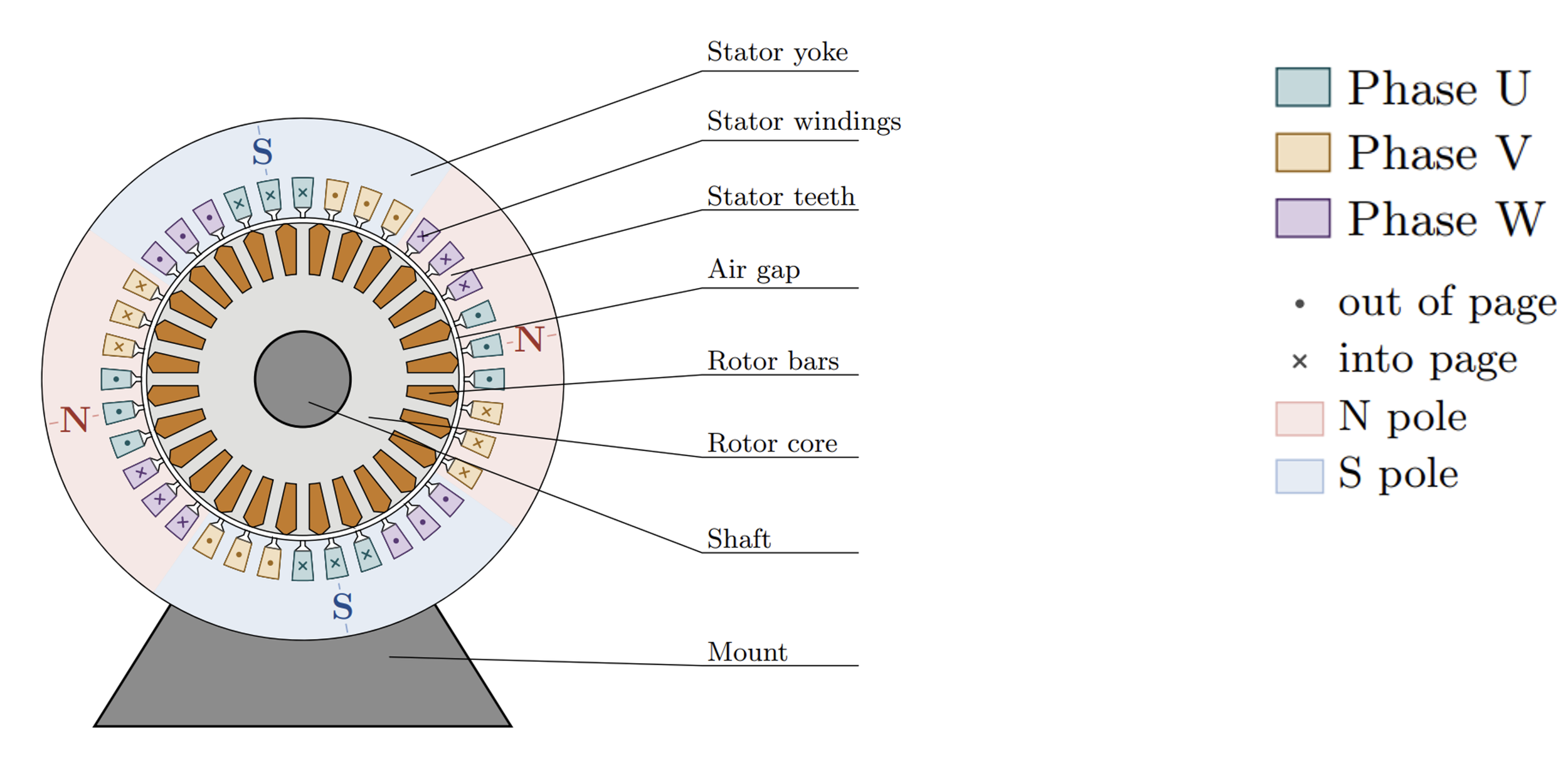
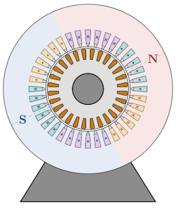
The only added information in this diagram, comparred to the CAD drawing above, is the dots and x’es. These indicate the direction of current in the windings. We are also showing the pole designations; 2 red north poles and 2 blue south poles.
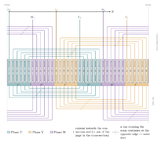
Below is the winding diagram showing how those are connected. The diagram has cut the rotor and rolled it out on the floor so that we see it from the top instead of a cross-section view as above. If you like, you can print it and tape it together in the “seam” to restore it.
All the lines outside the slots are the bundled mess stringed together which one can see when opening a motor.
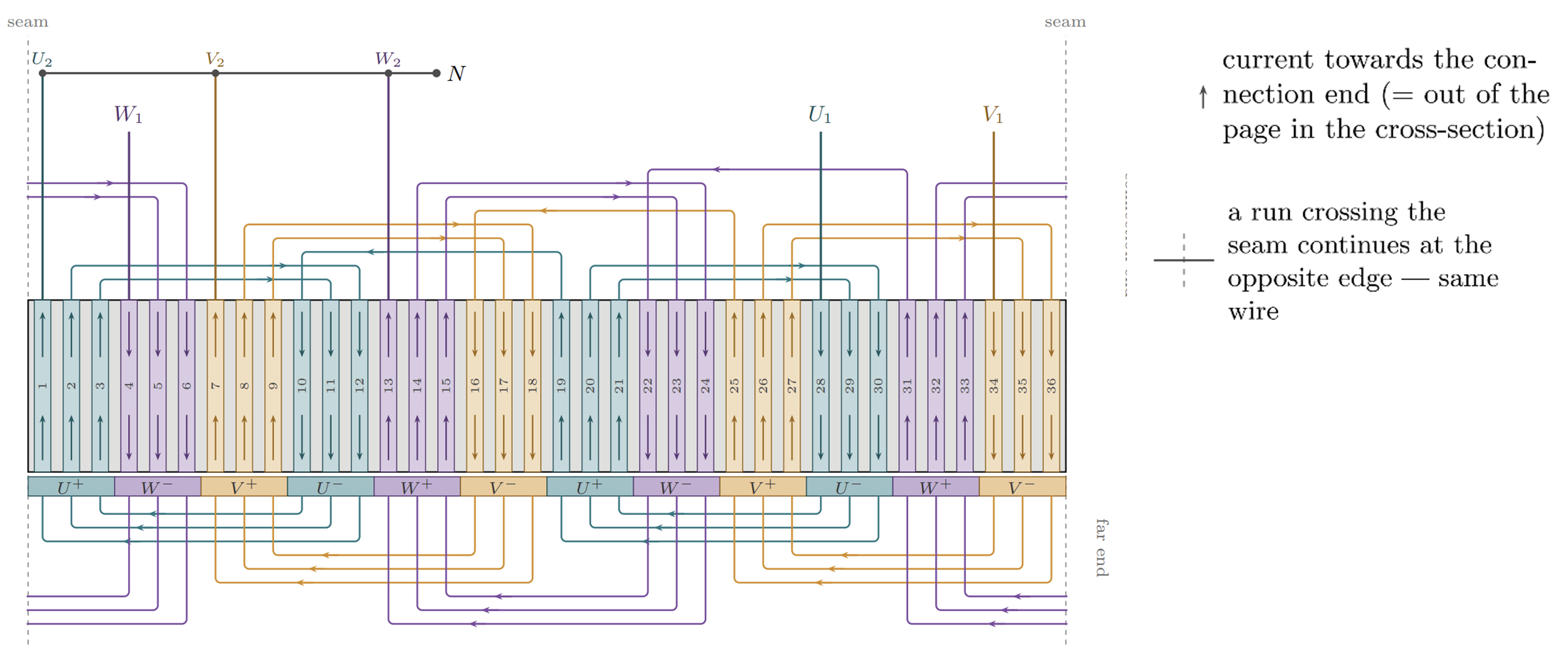
In a real motor, there is more than one turn on each winding, just to be clear on that.
More variations
Below is the same view of a two-poled motor.
It is a little less common in use, but when learning how it works it gets easier because the whole stator performs one revolution of the magnetic field when the electrical supply performs one revolution electrically. Each added pole-pair reduces this, and one must do a mental adjustment to take that into account.
With 2 poles, this is not necessary.
Where does the rotation come from?
If you ask a kid what he makes of the rotor or stator, why will probably say “round” or even “circular” if well-articulated. And yes, they are both quite round. But that does not explain why it rotates. There has to be a rotating field, not a circular one. Something need to spin, can we agree on that?
So let me introduce to you some of the old tricks from the three phased systems you probably learned at power engineering school but never cared too much for:
Space Vectors.
The first thing we should point out, in case you’re really rusty, is that in a three phased power system there are three voltages. When you take their instantaneous values (i.e. magnitudes) and add them together, you get zero (as long as everything is balanced and healthy).
But there is another way to add them too; vectorially.
This is possible because they oscillate between a minimum value and a maximum value - but not at the same time! They are phased-offset by 120 degrees each. And because the voltage is time-varying, that means that the phase offset is also a duration. In 50 Hz, a full cycle is 360 degrees and lasts 1/50 seconds, i.e. 20 ms.
If we take 120 degrees of those 360 - we land at about 6.67 milliseconds between each phase. So if phase U has a maximum at T=0, then phase V comes 6,67 ms after and W comes about 13 ms after phase U. This is very useful for us, because if they all oscillated in sync, then we would have aweful lot of trouble getting an induction machine to rotate.
So, allow me to re-use an old animation friend of mine, now with updated colors for the occation. Namely, the rotating 3-phased animation:
What we see here, is the reason why three phased supplies are so darn useful in machines:
On the left side we have a circular vector diagram showing the three phases at their respective angle and magnitude - increasing towards max, and shrinking to min. At the tip of phase U there are two small “helper-vectors” of phase V and W to illustrate that the black long space vector indeed is the vector sum of all three phases. Notice that its length is constant even though the three others are changing all the time. This is because the vector sum is always 1.5 x the amplitude of the three phases, whereas the arithmetic sum (without angles) is zero.
The same information is shown to the right, but as sine waves. Each phase has its own sine wave - they are locked in phase but their amplitude change with time. The moving vertical bar shows the vector sum when at its peak, and at the same point in time as the rotating diagram.
“hmmm… OK.. that circle does indeed remind me of a stator, and with the phases at different angles and a resulting rotating vector I think I understand where you are going with this” you might think.
So lets go there.
Below, I have put the entire rotating vector diagram into the machine and with the windings located just outside in the stator, you can see how installing the windings in an alternating and circular fashion also produces a steady, rotating resultant vector inside the machine.
Notice how it points to the windings which has the highest amplitude and direction inward (dot). The south pole sits at the opposite end for the current coming out of the rotor (x).
This being a two poled machine makes a very direct translation between one mechanical revolution and one electrical revolution. At 50 Hz, the stator synchronous speed is simply 50 Hz times 60 seconds equals 3000 rpm. The actual motor rpm is typically a few percent slower due to slip. Slip is covered extensively later.
Adding one more pole pair makes one mechanical revolution spend two electrical ones, so we should update our equation to take that into account: synchronous speed is now (50 Hz times 60 seconds) / divided by 2 pole pairs. Which is 1500 rpm. There. Nice.
Here is how it looks:
Above, I removed the three phasors in the internal vector diagram and instead just display the resultant vector.
But wait! There are two of them now! Of course, because there are two sets of windings installed 180 degree apart from each other in the stator, and both of them produce a rotating field - also 180 degree apart. How clever.
What about three pole pairs? How would that look?
Say no more, here we go at 1000 rpm synchronous speed:
Isn’t that beautiful? We have three resultant vectors now, 120 degree apart.
“But what about the winding layout, how does that look when animated”?
I got you covered:
Below you can see the 2 pole pair stator once again, but rolled out.
Now, the 36 slots are visible top-down in all their length, and inside each slot you can see the winding current (or voltage; in this animation you can choose), and the length and direction of the arrow is the current moving through. You also see the travelling wave underneath, labeled air-gap MMF. We will soon proceed to explain that, but for now we suffice with the acronym: MagnetoMotiveForce.
So far, I have presented voltage and current, the windings in the stator and how they produce a rotating change of amplitude, and a vector sum which is constant in magnitude and rotates evenly around the circumference of the stator.
But what about the rotor? What about the magnetic field? And the mechanical rotation?
We will start to dig into that now. They all come out at the same time when we start poking at them, so we will take our baby steps to ensure each aspect is well understodd (and illustrated or animated).
The magnetism
The stator and rotor iron. The different parts of the iron has different reluctance (magnetic “resistance”), and the airgap itself is an enormous one. The force driving the magnetic field is called MMF, and is created in the slots by the windings / rotor bars.
The beautiful circle above is our beloved stator and rotor yet again, but this time as a FEM-analysis showing the magnetic field lines. The field lines exist in all parts of the iron such as the yoke, the teeth and so on. These parts have different reluctance. They are small compared to the air gap, but not negligible (the teeth are the ones that bite).
The MMF arrow is pointing at a winding slot, trying to explain that the magnetic driving force is created by the current in the windings that reside in those slots (and in the rotor bar slots).
MMF is quite simply the product of current and the number of turns. If you want a magnetic field of a given strength, you calculate the reluctance in the loop and obtain how much MMF you need. Then you add current and turns until satisfied.
This sounds very much like electric circuit theory introductory course. If you want a given current, find the resistance in the loop and add a voltage source according to Ohm’s law and we are done.
The magnetic equivalent circuit. Fancy style letters, but other than that, it is just like an electric circuit.
Subscripts are: ts=teeth,stator - g=airgap - tr = teeth,rotor - cr=core,rotor - ys=yoke,stator
Above the equivalent circuit is shown. The observant reader will point out that this is a mirrored vertically where both the stator and rotor contain the same elements. They will also notice that the \(\mathfrak{R}_g\) is larger than the other reluctances. That is because the air-gap is the big and important reluctance to the magnetic field compared to the iron.
But the most important part to notice, is that the MMF on the rotor side is opposing the MMF on the stator side. Its polarity is reversed.
Essentially, we have that the MMF induced by the stator current is being opposed by the MMF induced by the rotor currents. This is important, and we will come back to it.
The unit of MMF is, quite simply, Ampere-turns. Multiply ampere by turns, voila, MMF.
The unit of reluctance is inverse Henry, \(H^{-1}\) or A/Wb. That is, Ampere per Weber. We have not discussed Weber yet, but that is the unit of magnetic flux.
The reluctance is calculated by \( \mathfrak{R} = \frac{\ell}{\mu_r mu_0 A}\), where \(\ell\) is the length of the magnetic material and \(A\) its cross section (not amps).
The \(\mu_r\) and /(\mu_0\) are the magnetic permeability of the material; how “easy going” it feels for the flux. Again, this is very similar to calculating the resistance of a copper conductor, isn’t it?
The reluctances has “MMF-drops” in the same way as impedances in an electric circuit has voltage drops. When you sum up all the voltage drops, you obtain the supply voltage. Thus the sum of “MMF-drops” across a magnetic circuit is also equal to the induced MMF.
An important difference between magnetic circuits and electric circuits is that flux which is opposed by reluctance, does not generate heat. Flux also does not flow like current does. It just, exists.
When designing the machine, the designer need to know exactly how the MMF is being distributed in the different parts of the iron to make sure that the resulting magnetic flux gets strong enough to create sufficient torque, but also leave enough margin to prevent that the iron saturates.
Magnetizing the iron
I did not originally intended to include an in-depth explanation of how the iron respond to the magnetic field, but during my research for this article, I found that this insight is actually quite interesting. Please forgive me for bringing us well into the turf of material scientists, but we are going to understand this magnetic field thing, aren’t we?
And yeah, it took almost three extra weeks getting this right. And even tough it is not specifically what Charlie asked for, I hope he finds it useful in his quest to grasp the field weakening.
I also want you guys to end up with a mental picture where you are picturing the machine’s space-vector sweeping across the circumference while affecting the iron, like a perpetual circular row of falling domino bricks as if they are in orbit around the rotor. Well, maybe not that vivid, but almost.
The main outcome from this section should be that the winding’s magnetic field alone is tiny, but can do great things with the help of iron. And that the iron has a limit, a limit every machine designer must know.
Magnetizing Iron
Have you ever wondered why iron is used when building electromagnets in the first place? Earlier I was under the impression that iron was pretty good at keeping the magnetic field “in place”, almost as a magnetic flux conductor. Well, yes it is, but it is also something a lot more significant.
The most impressive reason iron is used is that it comes with included magnetism. It just needs to be unlocked.
You see, the magnetic field from the winding alone provides a very modest magnetic flux density. The winding by itself is nothing more than an air coil where you get milli-tesla, and milli-tesla is not going to give us any meaningful amounts of newton-meters on the shaft.
The real trick here is that inside iron there are already countless, miniature magnets we call magnetic domains. These are defined regions inside the iron which themselves are magnets; i.e. fully magnetized iron - but initially with random north-south directions. Iron is not just one big crystal. It's more of a mosaic of tiny crystals called grains, each with its lattice pointing whichever way it happened to grow, and each grain hosts its own set of domains.
When adding them up in this state, they simply sum to zero. That is why iron by itself is not a magnet. We need those domains aligned. And this is what we achieve by imposing the tiny external magnetic field from the winding.
When this alignment occurs, we get a gigantic magnetic flux density, several thousand times stronger than our tiny winding-generated field would have made on its own. With stronger and stronger current, their consolidated contribution increases sharply in the same direction as our winding field. It’s an amplifier.
First we had an aircoil, now it is suddenly “buy 1, get thousands for free”. It is practically field day: A fire sale of magnetic flux density. What you are buying with is H-field (which you get from your amperes), and what you get is a ridiculous amount of flux density (Tesla) in the iron.
We use millitesla from the winding and get actual whole teslas from the iron.
What happens physically is that when the sine wave of the current is oscillating, the tiny magnetic domains are responding in the iron. The “favorable oriented” domains, pointing closest along the H-field’s direction, grow in size and occupy the volume which the non-favorable ones are leaving behind when shrinking.
This is the first, and “cheapest” mechanism and is called “wall motion” (as the walls of the magnetic domains appear to grow into their neighbours).
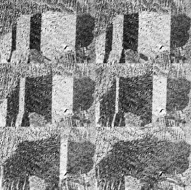
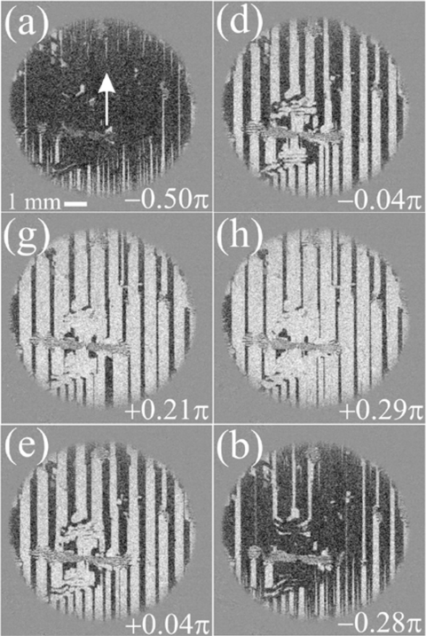
Below there are two real-life kerr-microscope image-sequences showing how the magnetic domains are “recruited” when an external field with vertical direction is applied.
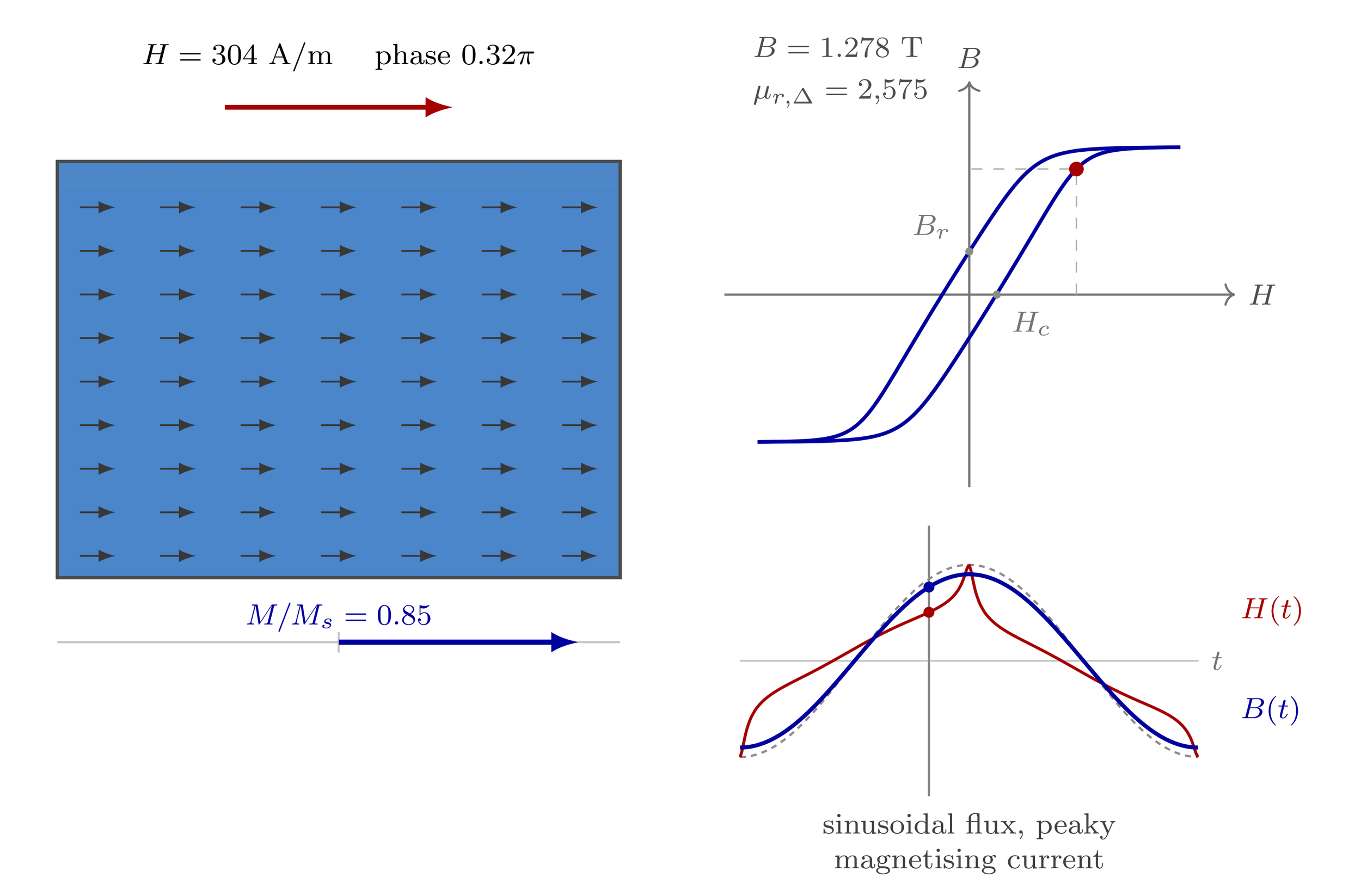
A schematic version is shown below. The domains are shown as a grid of arrows, and together I have drawn a BH-curve in the upper right corner, and the actual sine wave of both the H(t) and B(t);
the H(t) is the magnetic field strength in ampere per meter.
the B(t) is the magnetic flux density you get in tesla.
the \(\mu_{r,\Delta}\) is the slope, i.e. how much “extra” flux density you get per ampere.
M is the magnetizing of the iron, where \(M/M_s\) is how “saturated” the iron is. We get more into this shortly.
You may ask why the BH-curve is not a simple line instead of a curve with an area inside. In short, the area inside that curve is the hysteresis loss - energy spent influencing the iron by changing these magnetic domains back and forth. This is real heat loss as joules per cubic meter of iron, per cycle as domain walls are snagging on defects and grain boundaries, then break loose in sudden jumps, and each jump dumps its energy as heat.
Reaching the iron’s limit
When something is heavily discounted, it is tempting to get as much as possible.
But every fire sale runs out. Applying more and more current works well until most of the magnetic domains are lined up. Adding more current now reduces our yield for more flux back toward “buy 1, get a few extra”, and when we are used to getting thousands, this is not worth in anymore; there are current limits to uphold to, both in terms of what the winding can actually take before the insulation starts to smell weird, and the actual current supply from the inverter or mains. On top of this comes RI² losses.
Squeezing those last tesla out of the iron is either not possible due to thermal constraints of the windings, or by current limitations. Theoretically, we can, but practically, economically and sensible, we won’t.
Saturation in iron means that spending more current to increase the magnetic field strength has a very little effect on the magnetic flux density you get in return. The flux density you already have is kept though, but increasing it requires too much current to make sense.
You might have figured this yourself already: As you keep staring at the animations, you realized that there is a finite amount of magnetic domains to recruit. At some point each grain has just one big domain left. But it isn't pointing at our H-field, it is pointing along one of six directions set by the crystal lattice, whichever of them happened to sit closest. And since the grains are randomly oriented, "closest" can still be a long way off. The last effort is to rotate the direction of that domain.
This is the expensive part, and here is where saturation begin to play its part. The reason for the cost difference is that wall motion just moves a boundary while rotation means dragging the magnetization off the crystal's preferred axis and the crystal is pulling back hard. I could spend another ten paragraphs about this crystal-lattice stuff, but I think we are far enough down into this rabbit hole.
Let us instead expand the animation to include saturation and see how that looks:
What we see now is that:
The BH-curve got bigger with a very flat section and the top and bottom
The H(t) curve looks pointy - hmm… let’s get back to this one
The H required increases a lot while \(\mu_{r,\Delta}\) returns almost no flux density
Typical steel datasheets quote \(\mu_r\) as B/H measured from the origin, which stays quite high long after the “local slope” has given up. My μ_{r,\Delta} is the local slope, which is the honest one. It is how much more B do I get per unit H.
Let me explain this pointy H-curve:
Our winding above is voltage fed. Voltage is effectively locking the flux linkage \(\lambda\), so B(t) has to stay as sinusoidal as the voltage, whatever the iron thinks.
When the flux is peaking, the iron is well into the knee of the BH-curve and \(\mu_{r,\Delta}\) has collapsed from thousand-something to dozen-ish. The only way to deliver the B which the voltage demands is to throw enormous amounts of H at it. So H spikes into literal horns at the peaks, while staying close to normal in between. Because H is proportional to amperes, this pointy trace is the magnetizing current waveform.
In a real machine on mains or an inverter, saturation never shows up as flattened flux. Instead, it shows up as ugly current with pointy waveform. The B–H curve gets drawn in every textbook, and almost not a single one of them tells us what saturation actually looks like at the terminals.
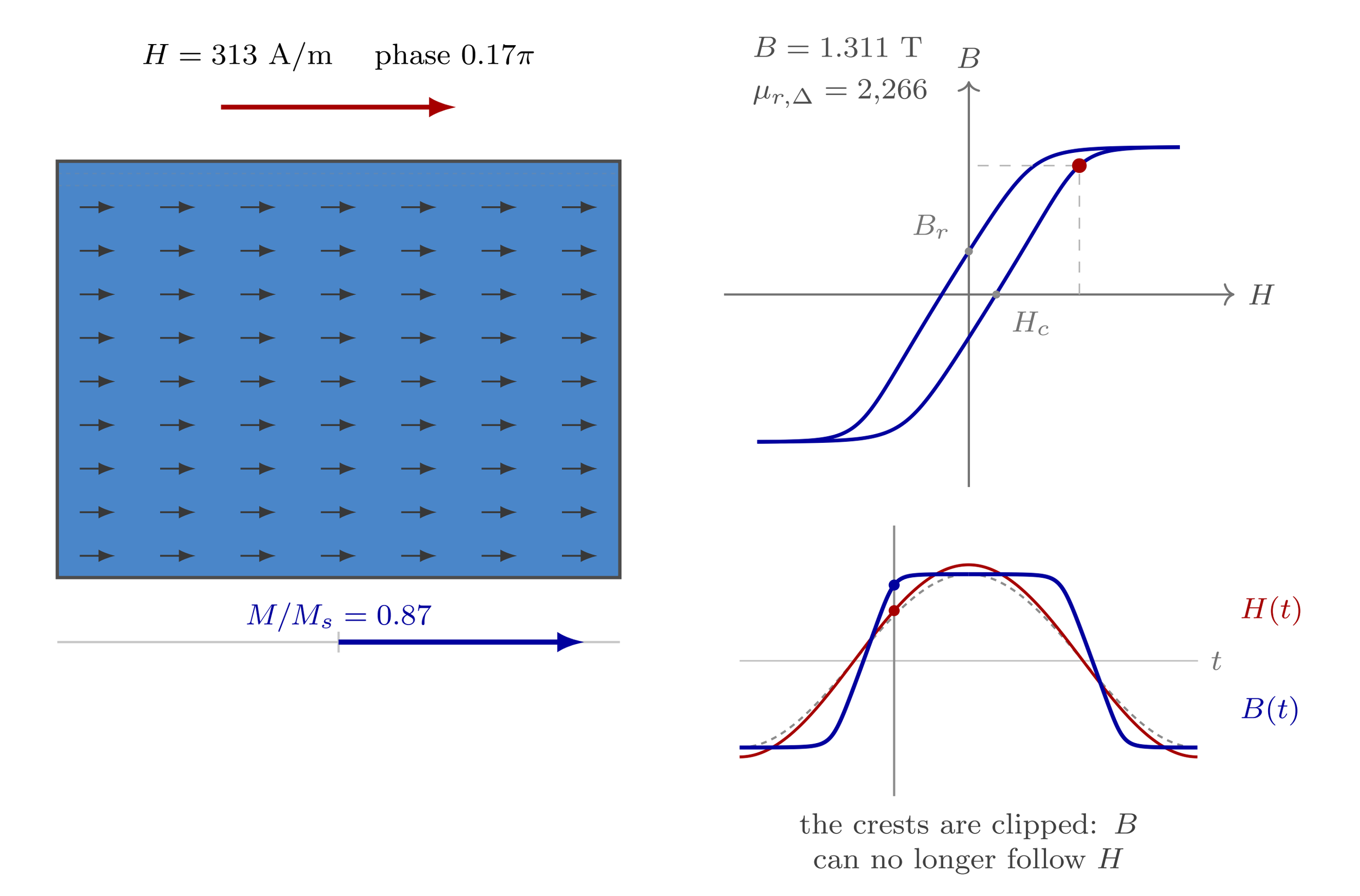
If, however, the winding was current-fed, meaning that current is controlled (i.e. not affected by the circuit or any other interfering phenomena in the iron), this would have been a whole other story. You might have seen this in FEA-tools which typically control current instead of voltage.
In a current fed winding, you impose a sinusoidal H and B flattens while current stays a clean sine. Both pictures are right, but they are controlled by a different “free variable”. The most usual in real life is the voltage fed one.
[Short pause while the agony from never seeing these graphs in the textbooks slowly diminishes]
OK.
Let us summarize some terminology while you have seen some of it in action:
The relative permeability, \(\mu_r\) is “how much more” magnetism you get per amp, and for iron this value typically sit somewhere between 2000 and 5000.
\(\mu_0\) is the permeability of vacuum, (i.e. how much magnetism free air “permits”) given as \(4π10^{−7}\) in Henry per meter. \(\mu_r\) is a material’s relative permeability compared to \(\mu_0\), so for example 4500 is a kind of a multiplier (the fire sale; buy 1 get \(\mu_r\) for free).
\(\mu = \mu_0 \mu_r\): This is the slope of the BH-curve, and varies somewhat during the slope (it looks linear, but just almost). Different types of iron is usually listing their maximum value.
\(\boldsymbol{H}\) is the magnetic field strength we buy with current, its unit is ampere per meter; A/m.
\(\boldsymbol{H} =\frac{\mathfrak{F}}{\ell}\), ergo divide the MMF by the length of the material to see what field strenght we have in that length.\(\boldsymbol{B}\) is the magnetic flux density we get in the iron, its unit is Tesla. As flux is Wb and density is cross-sectional, we get that \(T = \frac{Wb}{m²}\).
\(\boldsymbol{M}\) is how much the iron is magnetized. This is the one reaching its limit when saturation occurs. Let us derive its unit, shall we?
\(m=I⋅A\) tells us that an itsy-bitsy-tiny current loop with current \(I\) and loop area \(A\) creates a moment \(m\). This is not a Kodak moment type of moment, but related to an electron’s spin.
Now, the term Magnetization, is defined as “moment per unit volume”: \( M = m/V = I⋅A / V \). In units, this become: M = Ampere⋅m²/m³ = A/m. Ampere per meter.
Wait, that sounds familiar!
\(\boldsymbol{H}\) is having the SAME unit. This is a super-important insight! The units match because a magnetized lump of iron is, from the outside, indistinguishable from a coil of current wrapped around it. The domains are current loops. That's why they can add directly to H; they’re the same physical quantity, one from wire, one from electrons in iron.
So we apply the H-field and get thousands of extra miniature M-fields to help us out.
Let us see how this works out when run some numbers on it:
The flux density \(\boldsymbol{B}\) we get in the iron is
\(\boldsymbol{B} = \mu_0(\boldsymbol{H}+\boldsymbol{M})\)
Yeah, this makes sense. We get B from both our little H and our big M.
Adding some real actual steel for realism: M400-50A is a type of “cold-rolled non-oriented electrical steel grade designed for efficient magnetic core performance in electrical equipment” - sounds perfect. Just a quick one on what its name means, it might come in handy one day:
M: magnetizing iron,
400: Maximum iron loss (core loss) of 4.0 watts per kilogram at 50 Hz and at 1.5 Tesla.
50: Sheet thickness of 0.5 millimeters.
A: Non-oriented grain structure, meaning magnetic properties are (roughly) equal in the plane of the sheet. This is what we want in a motor where the field rotates and there is no single favoured direction. A transformer is the opposite case: the flux runs the same way through the yoke every cycle so the grains are deliberately lined up with it. This gives us both lower losses and more usable tesla.
Ok, so M400-50A has a magnetic polarization, \(J_s = \mu_0 M_s = 2.0 T\).
Its magnetic saturation, however, is
\(M_s = \frac{J_s}{\mu_0} = \frac{2.0}{4 π 10^{−7}} = 1.6 ×10^6 A/m\).
That is 1.6 million ampere per meter which the iron supplies almost for free. This is exactly the fire sale I was describing above: buy 300, get 1.6 million.
In the animations above, the H-field from the winding was about 300 A/m just below the knee area. Note that there is no knee “point” as some literature calls it, it is actually quite rounded. Maybe more like a “knee curve”.
An examle of a typical non-oriented steel datasheet which lists the flux density at different A/m illustrates this. I also added the difference between \(\mu_r\) which the datasheets sell, and the \(\mu_{r,\Delta}\) that matters:
1.29 T at 300 A/m - \(\mu_r\) = 3450, \(\mu_{r,\Delta}\) ≈ 2575 (read of the curve of the animation)
1.53 T at 2 500 A/m - \(\mu_r\) = 487, \(\mu_{r,\Delta}\) ≈ 32
1.63 T at 5 000 A/m - \(\mu_r\) = 259, \(\mu_{r,\Delta}\) ≈ 32
1.75 T at 10 000 A/m - \(\mu_r\) = 139, \(\mu_{r,\Delta}\) ≈ 19
These last ≈0.10 Tesla increments require more and more amps per meter. While in the non-saturated region, 300 A/m gets us to around 1.3 T, which is both much more comfortable and affordable.
The resultant flux density from the iron and the winding then becomes:
From iron: \(\mu_0 × 1.6 × 10^{6} ≈ 1.3 T\)
From winding’s H-field: \(\mu_0 × 300 = 3.8 × 10^{−4} T \)
So, around 1.3 Tesla from the iron and a tiny weeny 0.00038 T directly from the winding.
A very small push unleashes a lot of flux density in the iron.
The guys in charge
The magnetic state in the iron is governed by two guys:
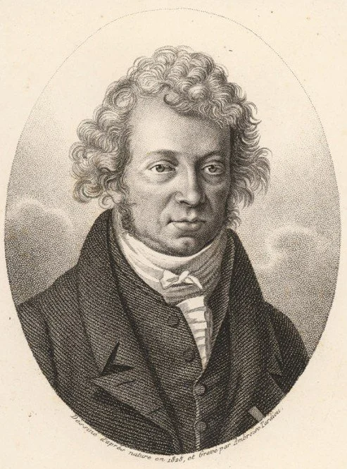
André-Marie Ampère, a French mathematician and physicist (1775 - 1836)
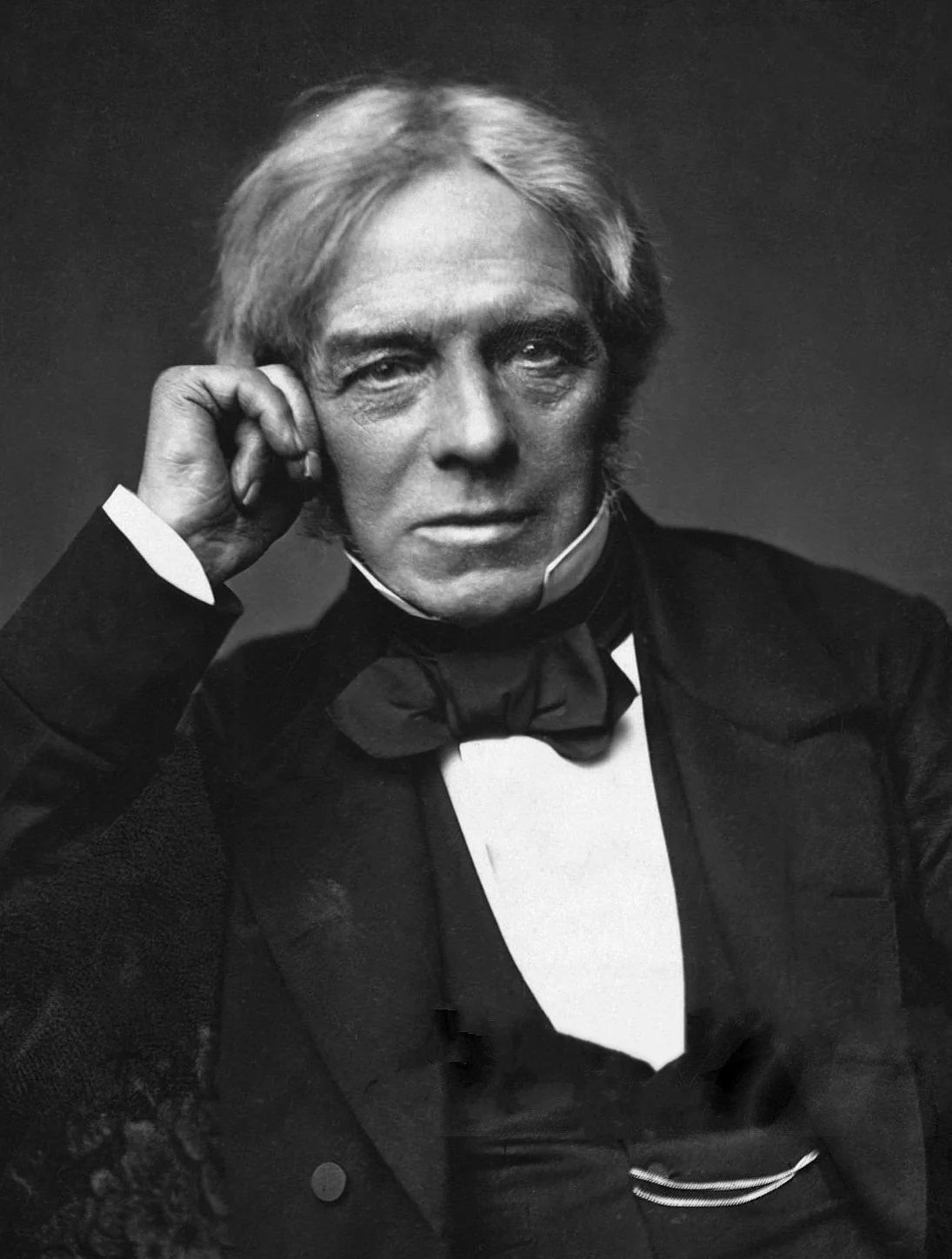
Michael Faraday, an English chemist and physicist (1791 - 1867)
There are two laws named by them, and they hold true simultaneously - always:
Ampère: \(N \cdot i = \boldsymbol{H}·\ell\) — the winding current sets H
Faraday: \(v = N \cdot \frac{d\Phi}{dt}\) — the terminal voltage sets dΦ/dt
You can't pick one. The magnetic state is a single state inside the iron, and both equations describe it. What changes is which variable your circuit locks and which one is free to land wherever it must.
This means that one of them sets the reference for the other, and which one is decided by our choice of control: Either we dictate the voltage, or we dictate the current.
In most applications, the voltage is the one we dictate; either fixed voltage from an outlet, or from a VSD which is synthesizing a voltage for us when controlling the motor. In this scenario, the current is the result of voltage.
In other settings, current is the controlled variable. Typical in industrial electro magnets, or DC choke applications or in older thyristor inverters. Here, the voltage changes to accommodate the current we dictate.
When current-driven (Ampère decides): We enforce \(i\).
So \(\boldsymbol{H}\) is fixed and \(\boldsymbol{B} = \mu \boldsymbol{H}\) follows, and \(\Phi = \boldsymbol{B}A\) follows. Voltage is the dependent variable; whatever the ramping flux happens to induce.
When Voltage-driven (Faraday decides): We enforce \(v\).
So \(d\Phi/dt\) is fixed, and \(\Phi \)is pinned by volt-seconds. \(\boldsymbol{B} = \Phi/A\) follows from that.
Then \(\boldsymbol{H} = \boldsymbol{B}/\mu\), and current is the dependent variable:
\(i = \frac{\boldsymbol{H}\ell}{N}\).
The winding draws whatever magnetizing current is needed to produce the H that sustains the flux the voltage demands.
This is the reason why there are two different sine waves for B and H shown earlier, one for when the voltage is controlled (pointy H-curve) and one for a current controlled scenario (B is flat on top).
From terminals to iron
Ok, that was a detour.
From now on, we are controlling the voltage. No more current sourcing.
To understand what is going on when voltage is applied, you first need to understand that (again) there are two laws which simultaneously are true. Always:
Magnetic: The iron’s price: \(\lambda = \frac{N^2\cdot i}{\mathfrak{R}}\)
Electrical: The voltage source’s demand: \(v - R_s \cdot i = \frac{d\lambda}{dt}\)
(this is in fact the same law as Faraday gave us a few minutes ago, now with winding resistance included, and written in terms of λ = NΦ)
It is tempting to write a list where everything happens in a sequence; “voltage creates current, current creates H field, H-fields creates flux, flux creates flux linkage, which creates back-emf, which reduces current”, and so on.
But physics is not inclined to provide any sequence, it insists that many of these thing occur simultaneously.
For instance, once we send our supply voltage in the door to the motor, the back-EMF is already standing there - at full height - blocking the way. This is before the amperes have gotten anywhere at all.
Take a look at this diagram:
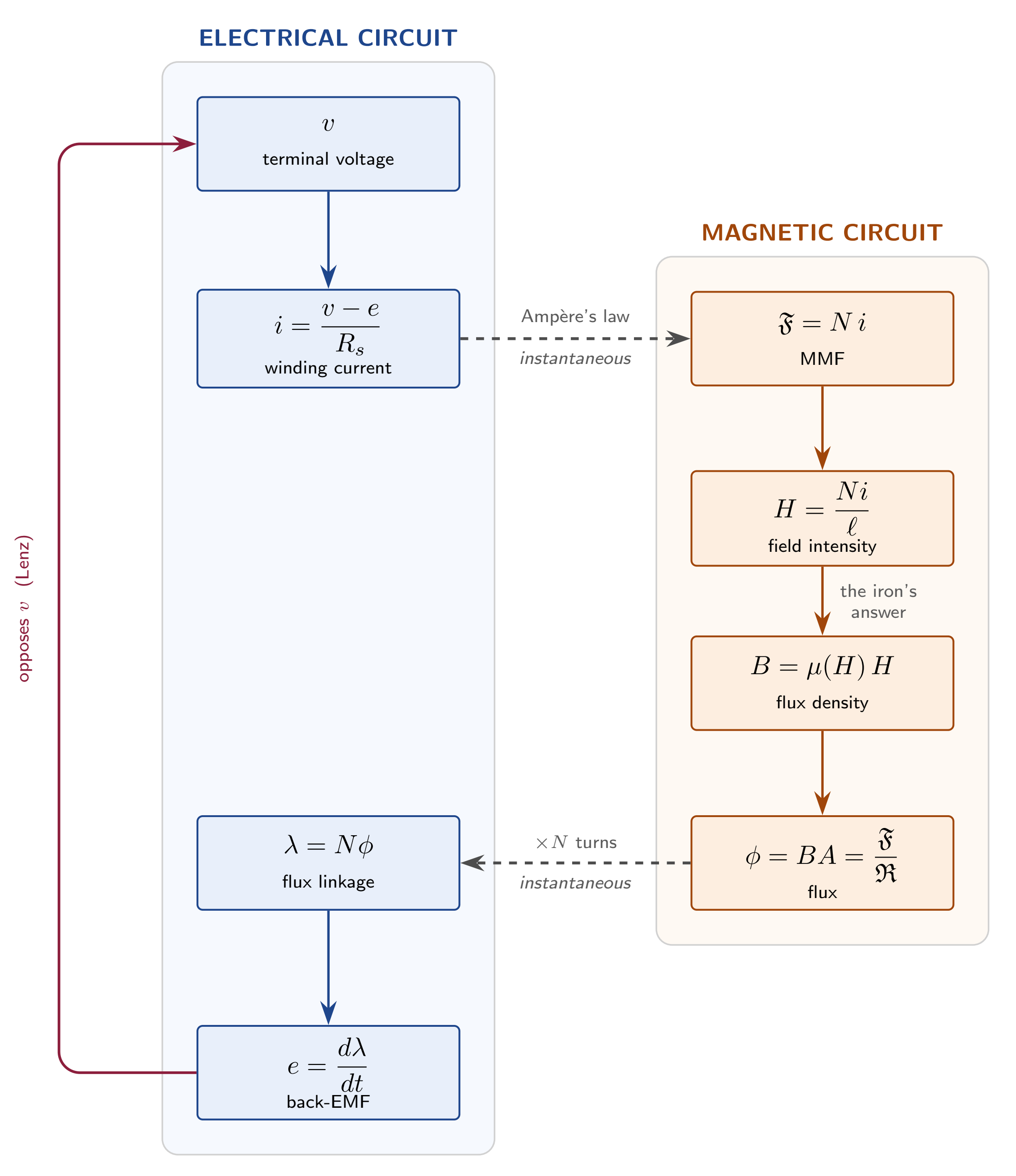
This looks like a flow chart - it is not a flow chart.
These events happen continuously, instantly and do not wait for each other.
The very instant you apply voltage, the back-EMF is standing right in front of you.
Even at t=0, when the current is zero, the MMF is zero, H and B are zero, even flux linkage is zero. But its derivative term is not zero. At t=0, the \( e = \frac{d\lambda}{dt}\) is at full force, making \(e\) instant.
Let us describe the figure a little more:
Terminal voltage \(v\) appears across the winding. The current that flows is whatever \((v−e)/R_s\) allows, and at t=0 that is zero
The current, together with \(N\) turns, sets up MMF:
\(\mathfrak{F} = N\cdot i\)When considering the iron as a circuit, it has a length, \(\ell\), and when the MMF is distributed over this length, we have the magnetic field strength:
\(\boldsymbol{H} = \frac{\mathfrak{F}}{\ell}\)When we take the iron’s properties into account, we get an amplification of magnetic flux density which we covered in detail previously. Observant readers now notice that \(\mu\) is a function of \(\boldsymbol{H}\), because as we say, it is not constant.
MMF drives the magnetic flux \(\Phi\), in the iron. The driving force is given by the current amplitude and the number of turns, N. It is opposed by the iron’s reluctance similar to Ohm’s law:
\(\Phi = \frac{\mathfrak{F}}{\mathfrak{R}}\)
Another way to reach the same value is by:
\(\Phi = \boldsymbol{B} A\)The same windings which created the MMF in the first place are also feeling that same flux as it appears in the iron. This feeling, and its effect on the winding, is called “flux linkage”.
How much the flux linkage affects the winding is given by the strength of the magnetic flux and (again) the number of turns, N:
\(\lambda = N \cdot \Phi\)The changing \(\lambda\) is inducing voltage back into the winding. The voltage polarity is given by Lenz’s law, and it will oppose the original voltage causing the flux in the first place:
\(e =\frac{d\lambda}{dt}\)The \(e\) is the back-EMF. That is, a voltage induces flux in the iron, but the same flux induces “back-voltage” into the winding of opposite polarity. Hence “back-EMF”.
Because the winding resistance \(R_s\) is tiny, \(e\) ends up being very close to \(v\):
\(i = \frac{(v−e)}{R_s}\). The current is simply whatever the small difference between them permits.
The above scenario plays out almost instantaneously and is called Self-inductance; that the magnetic flux a winding creates in a magnetic circuit, is also affecting the very same winding which created it.
One more thing is important to underscore, because it haunted me for years and impeded my understanding of electro-magnetism:
Magnetic flux, Φ, belongs in the magnetic circuit. This is what is appearing in iron and air-gaps (but can essentially be anywhere regardless of windings or electricity).
Flux linkage, λ belongs in an electrical circuit. This is how much a magnetic flux affects an electric circuit, typically a winding:
Consider a transformer with 100 turns on the primary side, where the primary side current creates MMF forcing a flux in the iron. There is only one flux in the iron. If the secondary winding has 1000 turns, the magnetic flux is linked 1000 times instead of 100, and the resulting secondary voltage is therefore ten times higher because: λ=N⋅Φ.
When flux links to a different winding than what caused it, it is “mutual inductance” and not “self inductance”.
Now for the punchline after all this magnetic babbling. Some of you might have wondered where I was going with this:
The whole magnetic circuit, every winding turn, every millimetre of iron path, the airgap, μ, all of it - they collapse into a single number the electrical circuit can use. That number is L. Our old friend, the inductance.
Check out below and see how inductance is defined. We should agree that inductance is important in an article about the induction machine:
$$
\begin{align}
L &= \frac{\lambda}{i} \\
&= \frac{N\Phi}{i} \\
&= \frac{N}{i} \cdot \frac{\mathfrak{F}}{\mathfrak{R}} \\
&= \frac{N}{i} \cdot \frac{N i}{\mathfrak{R}} \\
&= \frac{N^2}{\mathfrak{R}}
\end{align}
$$
These equations capture the bridge between the electrical and magnetic part of the figure above.
Notice how the \(i\) cancelled out entirely. It arrived twice; once from the electrical side in λ/i, once from the magnetic side in ℱ = Ni - and the two cancel. What's left contains no current at all, only turns and reluctance.
Point being: L is a property of the machine's iron and windings, not of how hard you might be driving it. And L is the price, because i = λ/L → Big L, few amps for a given flux. Small L, many amps.
Reluctance is the physical property of the iron; inductance is the same fact translated into terminal quantities which the electrical circuit can see.
In a few thousand words from now, we will have the machine’s equivalent circuit to discuss. That one consists of several inductances. Now you know that they are in fact made of iron and windings and what gave them their value.
We learned three things now;
how the voltage sets the magnetic flux in the iron of the machine, and
how the magnetic flux “kicks back” by inducing an opposing voltage by its own making, called back-EMF, and
how the iron cost is baked into inductances
The next thing we shall learn, is how that flux of ours are affecting the other winding in the machine. Namely the rotor bars.
The flux, the rotor bars and the torque
The motor is very much like a rotating transformer. Until now, I have only described what the “primary winding” in the stator is doing, completely ignoring our secondary “winding” in the rotor. It is not really a winding as it has no turns, also, it doesn’t look like one either. To me, it first looked like a creative short circuit. (Which is actually is).
So when our flux is passing next to the rotor bars, the flux induce voltage in them, too. The important thing here is that the rotor bars are at different places, and we have learned that the rotating magnetic field points in one direction at the time (the north-south axis). This means that the all rotor bars does not experience the same magnetic field simultaneously. Hence, the bars experiences different amounts of voltage induction. If they all got the same voltage, then there would be no current.
When the rotor is at standstill, the strength of the induction into the (closest) rotor bars are the same as the back-EMF:
\begin{equation} v_r = \frac{d\lambda}{dt} \label{eq:def_v_r} \end{equation}
That d/dt term is key here. I hate that “is key” expression, but in the induction machine - it really, really is The Key.
Everything about how a motor generates torque is conncted to how much the flux linkage is changing. This change can be detected and quantified and manipulated in two ways:
alter how often it changes during a period (e.g. by changing more slowly or by changing more often as in decreasing or increasing frequency )
alter how much it has to change during a period (changing the amplitude it has to reach within a cycle)
A visual guide to the fact that changing either the amplitude or the frequency will affect the d/dt term (the red tangent line).
So 2x frequency or 2x amplitude = 2x dλ/dt value.
The hat over λ is the peak value, in case you were wondering. The no-hat version is the instantaneous one.
Change is very important to inductance. No change, no induction. No motor.
I am stressing this because when, in a directly connector motor, the rotor is stationary and starts to turn, it will sense a very fast moving stator field. Just as if you are standing still and a car passes you at 100 km/h.
But when the rotor picks up speed, it will think the stator speed is slowing down. Almost as if you were accelerating up to 99 km/h next to the 100 km/h car.
This relative speed difference is super duper important, because if both the stator and rotor was synchronous, the rotor bars would have a \(dλ/dt=0\) which means no induced voltage, no current. The rotor would be inert. The only way to achieve this in reality, is to increase the speed of the rotor from the shaft by another torque than the motor provides. The motor itself cannot do it.
OK, back to reality:
Voltage is now being induced in various ways across the rotor bars, current is flowing in our squirrel cage. Guess what the current does?
It is setting up its very own \(F_r=N⋅i_r\).
This is the opposing MMF we saw in the magnetic circuit illustration. This MMF has two important attributes: magnitude and direction. These are individual and separate, which is a very important to what comes next:
Firstly, the magnitude: the rotor MMF counters the stator MMF. This would reduce the flux in the machine, right? No - because the flux in the machine is decided by the supply voltage (as we have learned recently). The very instant the flux attempts to drop, this is compensated by the voltage because suddenly the back-EMF drops, which increases the stator current, which increases the flux, which restores the original flux. This flux now costs “more current” as it is needs to cancel the rotor MMF. The motor now draws more current to uphold the same flux, because it also has to “pay” for the countering of the rotor MMF
Secondly, the angle. Because, by now, we have an electro-magnet. Which way is the magnet pulling? Well, it is trying to pull the rotor into the stator - radially the whole way around. Luckily for the bearings, the force is equal radially around the rotor, so the net force sums to zero, but the local force on the rotor teeth are quite high (in the order of several kilos per square cm on each tooth).
But this electro-magnet is doing no actual work. It just sits there, full of tension, trying to pull something that just doesn’t move.
And it does not move because the magnetic field lines are perpendicular between the rotor teeth and stator teeth. Like rubber bands again, trying to pull teeth toward teeth.
We need to change the angle of the force between the stator and rotor, and here comes the rotor-MMF’ second property in handy. Because rotational force is torque, and torque what the machine was paid to deliver.
Below is an illustration of what we use the rotor bars to achieve:
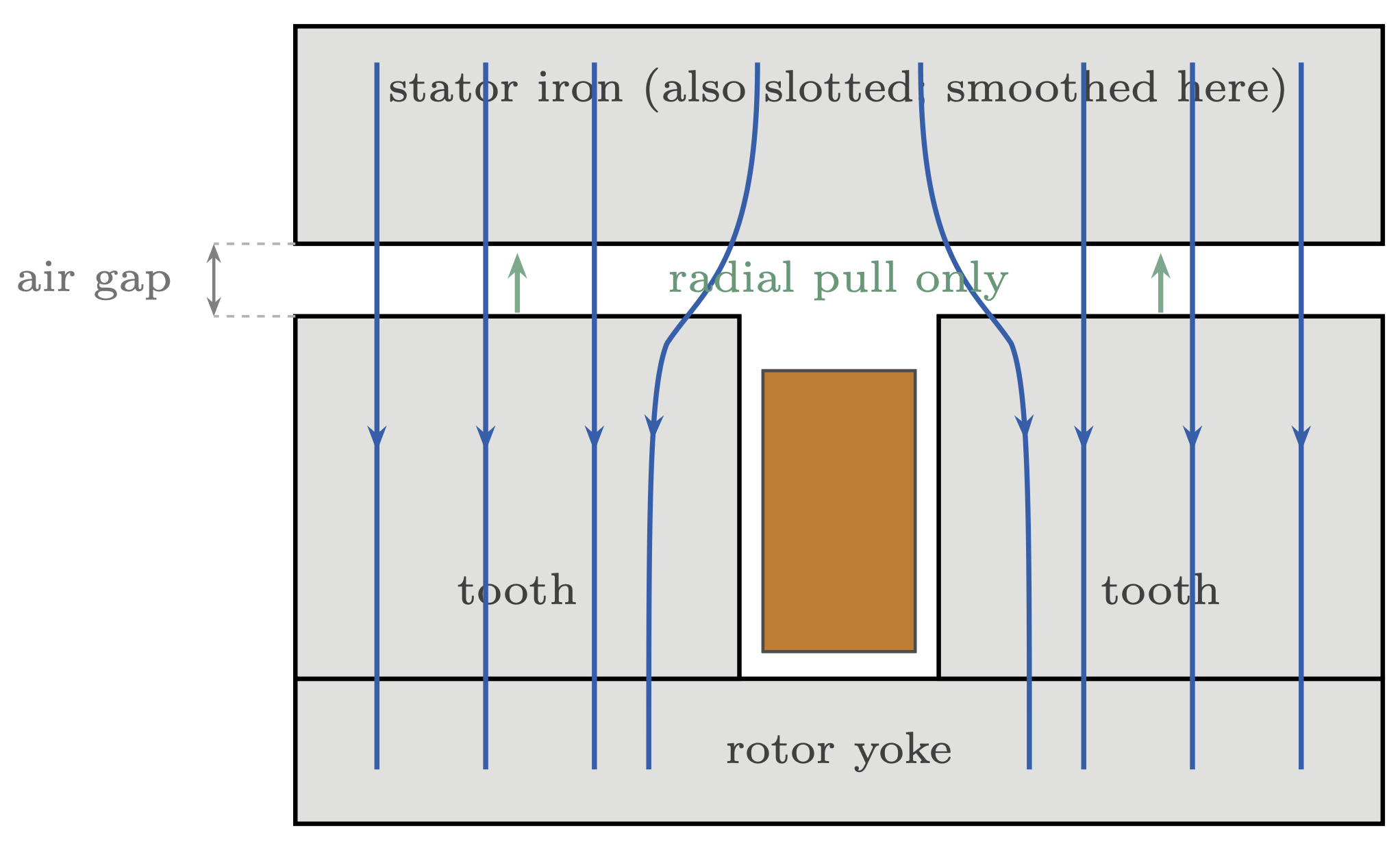
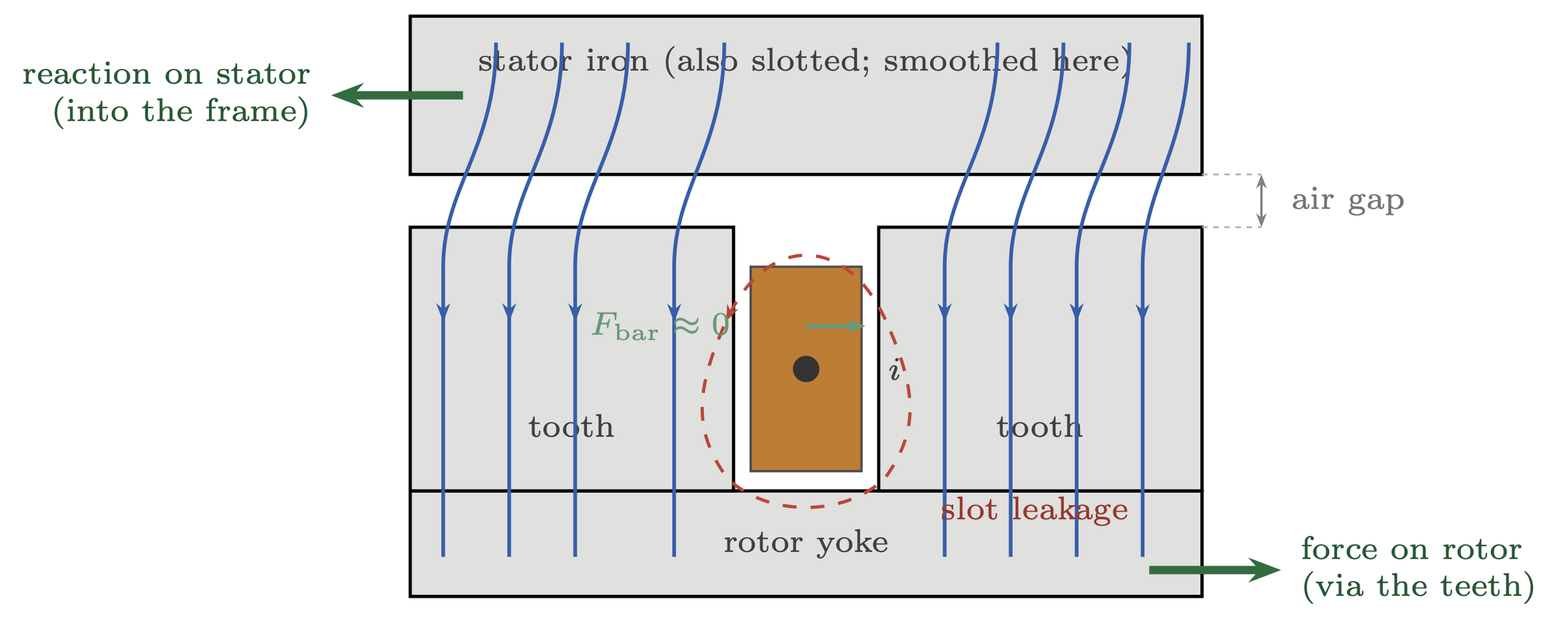
We see two versions of an air gap with the stator iron on top (shown without teeth here), and a cross section view of a copper rotor bar, the rotor teeth and the magnetic field lines.
At the left, there is no current in the rotor bar. The stator field is undisturbed and crosses the air gap in the shortest possible way. The force follows the field lines (remember, rubber bands), and tries to pull the two faces together.
At the right, current is flowing in the rotor bar, and that current creates its own MMF which distorts the existing stator field. The angle of distortion is exaggerated to get the point across, but you should be able to imagine that the skewed rubber bands are now trying to pull themselves sideways to restore the shortest possible crossing of the air gap. This creates a torque which acts sideways on the rotor teeth (and the stator teeth in opposite direction, but that can’t move can they?). The electro magnet of ours is finally doing some work.
Part 2 will explain how this happen. Stay tuned.